You are thinking about going to the Round Lake Wilderness for a Canoe Trip. You would like a map, but don’t want to spend $10 bucks to buy one, when you get a better looking map for free with more accurate data from the NYS Department of Environmental Conservation and NYS Department of Transportation, using a free GIS program known as Quantum GIS or “QGIS” for short. When you are done with this tutorial, you will end up with a map that looks like this.
QGIS like all GIS programs can seamlessly glue together multiple topographic quadrangles (such as the Sabbist and Little Tupper Lake quads needed for this map), and then superimpose campsites, trails, and other data you need — that might not be available on a typical topographic map. As your printing your own map, you don’t have to worry about keeping it dry or keeping it from getting damaged.
All GIS software is highly technical and a bit complicated to use. Putting together a good map is a fair bit of work, but once you master it, you will be able to put together quite nice looking maps. I hope this rather length fodder article will send you on your way to making good maps of NY State.
Step 1: Download and Install QGIS.
First you need to download a free copy of the open-source Quantum GIS program from QGIS.org. It runs on Windows, Linux, or Mac OS X and is relatively easy to install. Then open QGIS on up. It will look something like this, depending how many plugins you have installed and your version of QGIS.

Hint: Save your work regularly when working in QGIS by going to File -> Save Project menu. It’s always good to save regularly in any GIS program, as your dealing with large files, and its always possible that QGIS could crash, and you would lose your work.
Step 2: NYS DOT Topographic Index.
Next, you will need to get some data to fill up that blank screen. You will probably want to go the NYS GIS website and download the 7.5 minute topographic index (aka 1:24,000 scaled topographic maps). This “Shapefile” — a file containing data used to draw shapes, dots, or lines in a Geographic Information System (GIS) program — contains an overview map of NY State, with boxes representing each of the 965 7.5 minute topographic maps that make up NY State.
NY 1:24,000 Topographic Map Coverage Index Shapefile. (90 KB) Contains the outlines of all 965 7.5′ topographic maps in NY State. Freely available from NYSGIS Website, under the Digital Raster Quadrangles.
Download, expand, and open the NYSDOT Topographic Map. You can open it in QGIS by using Vector -> Add Vector Layer.

7.5 minute topographic maps are the most accurate topographic maps typically available. The NYS Department of Transportation provides high-resolution, 509 DPI, scans of all 965 topographic maps it creates. Each scanned in map is in a file called a “GeoTIFF”, and is divided into 3 or four files, consisting of each color used on a standard DOT topographic map.

It’s Very Confusing, BUT VERY IMPORTANT!!
When you load that 7.5 minute topographic index into QGIS, you might be surprised to see how that map is distorted, and does not look like the map above. This is because the earth is not a flat surface, and there are many ways to draw a map of the earth, to reflect the curvature of the earth. We call that the projection of the map — how we project a curved surface on a flat sheet of paper or a flat screen.
There are actually thousands of ways to project the surface of the earth, such as unprojected latitude and longitude (called WGS84) that squashes north and south on maps, regular Mercator which puts things on an even latitude or longitude on a flat plain (NY State appears with a flat border along Pennsylvania at the 42nd parallel), and Universal Transverse Mercator (UTM), which most accurately shows distance and relative position of items, at the cost of over distance appearing somewhat distorted.
For all your New York State mapping projects, you are only going to use one projection — Universal Transverse Mercator (UTM) Zone 18. This is one set in official state regulations as what all state agencies are supposed to use, and it’s what NYSDOT Topographic maps are drawn in. For your adventures in making maps for hiking, camping, hunting, fishing, and boating, your going to want to always use NAD83 / UTM Zone 18N in NY State.
Go to File -> Project Properties, and click on the Coordinate Reference System (CRS) tab. Browse through the list for NAD 83 / UTM Zone 18N. Click on “Enable ‘On the Fly CRS Transformation”.
Clarification. Then click the triangle next to Projected Coordinate Systems, then click the triangle next to Universal Transverse Mercator, then scroll down to NAD 83 / UTM Zone 18N (ESPG:26918). Alternatively on the search box on that same page, search for Authority: All, Search for: ID, and enter in 26918. QGIS will remember your settings and default to this projection for future projects.

To ensure everything is projected in NAD 83 / UTM 18N, make sure to Enable ‘On the Fly’ CRS Transformation. QGIS will automatically convert “Shapefiles” and other vector data into the proper projection. QGIS can not do this for scanned in images or similar “raster” data.
Check and recheck to make sure you did this projection step correctly. Otherwise, you will get messed up maps, and you will get lost. Confusing, definitely but the most important step.
Step 4: Now Let’s Load Some Data.
Shapefiles and vector data are all loaded in the same way. You download the file, expand it, and load it into QGIS. Here are some Shapefiles I recommend you download and load into QGIS:
DEC Lands Outlines Shapefile. (5.4 MB) Contains the outlines of all lands under the control and jurisdiction of the Department of Environmental Conservation. Does not include Town Parks, Canal Authority Parks, Parks Maintained by Office of Parks, Recreation, and Historic Preservation. Also does not include Conservation Easements. Freely available from NYSGIS Website, under the DEC Section.
DEC Roads and Trails Shapefile. (5.8 MB) Contains many of the roads and trails maintained by the DEC. Does not include local, county, or state roads, and in some regions of state, there is no trail data available. Freely available from NYSGIS Website, under the DEC Section.
DEC Physical Assets Shapefile. (0.2 MB) Contains many of the physical facilities maintained by DEC — specifically lean-tos, back country campsites, boat launches, fishing docks, firetowers, etc. This is available using a Freedom of Information Law Request. The DEC will send it to you in 5 days, if you email the Records Access Officer. I have put a copy of this file on my blog, of the exact form I got it back from the DEC, to allow you to avoid unnecessary FOIL requests.
OpenStreet Map: NY State Shapefile. (105 MB) I found this some time ago on a now defunct website and have made several modifications to it over the years. It is freely available data, originally based on US Census TIGER lines, but with certain modifications, such as removing certain roads from wilderness areas. One should consider it public domain as it’s just US Census data, and you are free to edit and redistribute it. You can download my copy from this blog.
Once you load the data into QGIS you should be able to zoom in and explore the map, and get a general idea of what area you are interested. The random colors chosen by QGIS to display this data are pretty hideous, but we will change them in a bit.

Zoom into the area you interested in, by looking at the general outlines of the public lands. You can use the maganifying glass to zoom in, the hand to move around, and the cursor next to the (i) icon, to display information about various features.

Step 5: NYSDOT Topographic Maps.
Next we need to figure what NY State Department of Transportation (NYSDOT) 7.5″ topographic maps we will need to make a “base” map of Round Lake. Click the cursor next to the (i) icon, then onto the the map, where you need to figure out what topographic map you want. As I see from the results, I will need the Sabbatist Quadrangle (among 4 others nearby), which is available from NYSGIS.

NYSDOT Topographic GeoTIFFs at 1:24,000 Scale. (2 MB per quad) There are 965 quads in NY State. The NYSDOT topos have the most up to date roads on them, and come with each color layer seperate. The average file is about 2 MB. I downloaded the whole set from their FTP site, but you can download only the ones you need at first, but having the full set sure is convient.
NYSDOT Topographic Maps are scanned at 508 DPI, and are georeferenced NAD 83 / UTM 18N GeoTIFF images, that QGIS will automatically position on map for you to create a seamless map across data layers, as long as you properly set the projection in QGIS in Step 2. Maps will line up perfectly, even a certain map consists of many different quadrangles.
I do not recommend the USGS Digital Raster Graphic (DRG) Quadrangles. They are typically older, use the obsolete UTM 18 / NAD 27 coordinate system, and do not have individual files for each color layer. Moreover, the 1:100,000 Digital Raster Quadrangles and 1:250,000 Digital Raster Quadrangles, do not have the needed resolution (detail) for doing hiking or other outdoor maps. If your doing a broad overview maps — like for spotting peaks off a firetower, they might be useful, but not for general use.
Each NYSDOT Topographic Map consists of 4 different black and white GeoTIFF images. There is no transparency data in this maps, nor any color in them. You are free to set transparency or color as you please. They are as follows:
- plan – Man made features and labels such as roads or mountain names. May also include unnavigable streams, borders on lakes, etc. Anything that would be printed black on the NYSDOT topographic map.
- hyd – Lakes and navigable waterways. Anything that would be printed light blue on the NYSDOT topographic map.
- topo – Topographic lines showing general elevation and slope. Anything that would be printed light brown (color of topographic lines) on the NYSDOT topographic map
- bua – Built Up Area, background. Areas that have a lot of development, such as cities. Anything that would be printed light pink or yellow on a NYSDOT topographic map. I usually don’t use this layer, not found in rural quads.
You can load them using the Layer Menu -> Add Raster Layer, menu item. Using the control key, you can load multiple files at one. I try to load all the layers I will need at once, as it can take time to load layers, and it’s good to get it done at once.

Remember, these are scanned in images or pictures of the topographic maps, they can not be easily edited or queried in QGIS. Zoom in too far, and they become pixelated. Yet, they usually provide an excellent back drop for outdoors maps.
When you first load one of these maps, you will see a picture like this. The topographic layers for some reason chose to load first, and appear on top, and with no color or transparency set, they are pretty useless out of the box.

Typically you will want to arrange the topographic layers, so that the plan layers are on top, followed by the hyd layers, then the topo layers, and finally the bua layers. With the plan layer up top, the map will start to make a little bit more sense, give you a better idea if you loaded the proper quads.

Next you will want to go through every GeoTIFF Topographic Map layer you have uploaded, and change white to transparent. You do this by right clicking on each layer, and choosing Properties. Then click on the Transparency tab in the Layers Properties dialog that comes up.

Double click on -32768.00 on the Indexed Value column, and change it to 0. This will make all white portions of the map 100% transparent. NYSDOT Topographic Maps do not contain any useful transparency data, so you will want to make all white areas in the map transparent.

If you are working on a hyd layer, topo layer, or bua layer, you will want to go the color map layer, and change the color for value 1.00000 by double clicking on the color next to it. Black is the default color, but that isn’t helpful except for the plan layer. You need not change the 0.0000 color, as you have already set that to be transparent, and it will not be visible on the map.

Then click OK, and the dialog will close, and transparency and colors will be visible on the map layer you just changed. Besides those awful background colors, the map that is being displayed starts to look a lot more useful now.

Right click on NYS_QuadIndex and choose Properties. Go to the Style tab. While we really do not have to use this layer any more, and could just disable it by unchecking it, I like to use it as a yellow background to indicate non-DEC lands on a map. To do this, click on the color box next to Fill Options, and set it to light yellow, as I did, or whatever color you want to represent private lands. Then go to Outline Options and choose an invisible line, to hide the quad boundaries.

It’s now starting to look a little better.

Now it we do the same with DEC Lands Outlines, setting it white or whatever color you prefer. Make sure it’s dragged above NYS Quad Index on the Layers, but below the Topographic Maps. I prefer no borders to be shown, as I find DEC boundaries to be confusing, as often Wilderness borders Wild Forest or Primitive Areas, leading to strange lines appearing in the maps. If you care about such borders, do leave them on though.

Now you got a map that is almost ready for use, that is once we delete roads that we know don’t really exist in a wilderness area, stylize campsites versus other facilities, stylize roads versus hiking trails, and maybe add some labels.

Step 6: Stylizing Roads versus Trails.
I like to make hiking trails a dashed black line of 0.75 map units, and roads a solid black line of 0.75 map units. This ensures on black and white printers one can tell the difference. To do this, right click on DEC Road and Trails, then the Style tab. From here, choose Unique Value from Legend Type.

We will use the MOTORV field to decide if something is a road or a hiking trail. Obviously, if this was a winter map, we might change this field to SNOWMOBILE or X-COUNTRY SKI. This field contains, ‘Y’, ‘N’, ‘M’, ‘U’, and sometimes ‘YES’, ‘NO’, depending on the forest ranger that inputed the data. Set the style as you wish.
Choose classification field MOTORV, then click the classify button. All of the different possibilities for roads or trails allowing motor vehicles will be shown. From there, set the colors and line styles as you so choose.
Step 7: Removing Invalid Roads from NYS Highways Shapefile.
If you use the OpenStreet Map Highway file future on the page, you will see it often has lines that overlap DEC hiking and truck trails, and has old woods roads or other invalid data, that you will need to delete to clean up your map, and avoid confusing users. It’s pretty safe to delete all highways from Wilderness-areas, unless you are sure that such a road actually exists.
You need to right click on New York Highways Shapefile, and choose Toggle Editing. A pencil will appear next to that layer. Then use the select tool on the second toolbar, in the upper left (selected in box below). Highlight the streets you want to delete, and they will appear yellow.

Use the Delete Selected button to delete the roads you have highlighted. Notice buttons nearby that allow you to split features into multiple features. These are helpful if you know only part of a road has been closed or abandoned, and you want to remove only part of the road from your map.

I zoomed in on Round Lake to search for other invalid roads I wanted to remove. Looks okay now, although I still question some of those roads located in Whitney Headquarters. Having not been there, I can not say which ones have been gated or abandoned, so I will leave them on for now. Right click on the NY Highways Layer to save your changes to that Shapefile.

Step 8: Stylizing Assets.
Next we need to change the various DEC Physical Assets from a single color dot, to icons that represent the asset. With the current map, we can not tell the difference between a campsite, a parking area, or trail register. This could be rather confusing for anyone using our map.

This is very similar to changing the symbols for roads versus hiking trails in the previous step. Go back to the properties dialog. This time, we want to stylize things based on Unique Value, then Classification field Asset. Then, click Classify. This will create unique color for each icon. By browsing the “Point Symbol”, you can now give primitive campsites proper looking icons. Don’t forget to set the size. I usually set icons at Size 3.0 or 4.0, but it varies a lot on the final scale of the map.

Finally, I zoomed in to check on my work. Wit the icons set, we have a pretty nice looking map. I can spot the campsites, parking areas, trails, and the private property-public lands boundaries. I know where to put in my kayak, to explore Round Lake. It’s too bad, I don’t know which if any roads to remove from Whitney Headquarters, so I’ll have to go in person if I want to correct the map.
Step 9: Adding Labels to Trails and Roads.
Yet, I would also like to see some names on the roads and trails. Select the DEC Trails layer. Go to Layers menu and choose Labeling. From here, click Label This Layer, then choose Fields with Labels and select Name. The default style of 12 point fonts is almost always too large for most maps, a font size between 5 to 7 points is what you mostly likely will use. Then select, Buffer to create a small white background around each label. This is usually necessary to make your labels appear readable on the map.

Then click the Advanced tab. The default placement for labels is Parallel, which labels the largest amount of items, but doesn’t look very pretty. Curved is the prettiest, but it will not label particularly twisty lines. Priority controls which labels are most important if you have multiple layered roads. I usually set NYS Highway Shapefile to a low priority as the underlying topos usually also have road names, and trails to a much higher priority.

So now you should be set with labels. You have to do this with each layer with labels, such as the NYS Highways layer. You can do this also with the assets layers, although I generally do not bother, as I don’t really care about the sometimes lengthy names the DEC gives campsites.

Step 10: Printing and Making Images to Export.
Looking at a map in QGIS is kind of fun, but pretty useless when your on the trail. Go to File -> New Print Composer. A dialog like this will appear.

Next, you will want to change the paper size to something more reasonable then A4. Most likely you’ll choose Letter-sized paper. Below that set the resolution. Choose the orientation most appropriate for your map, I often use Landscape. To get high quality map print outs, you will want to set the the quality box somewheres between 300 to 500 dpi. Even if you are just exporting as a picture, it is good to preserve the resolution for future printing.

Then click on the canvas icon (circled in blue), to draw the surface the map on your canvas. This will provide you a canvas to draw on your page surface. You may wish to click “Snap to Grid” and set “Spacing to 5.0” to make it easier to line the canvas up. Click the magnifying glass, with the plus sign or the icon directly to the left of it, to expand the window so it’s easier to work on the canvas. This doesn’t change output, only the display on the screen.

Next, click Item tab, and then the Extents label. This will bring up the map extent box. The extents of the map will be listed in Northing and Easting, a series of large numbers that tell you how many meters you are North and East of the Greenwich, England. This is the standard form of measurement used by the Universal Transverse Mercator positioning system. Just click, “Set to Map Canvas Extent”.

Click Map. You can use the Earth on Hand Tool (circled blue on this screenshot), to move around the image on the map. Then you can go to the scale box, and adjust the zoom. Smaller numbers mean more zoom in. A standard topographic map is at 1:24,000 scale, however, I generally prefer a scale of 1:18,000 or so to make the map more readable. If you zoom in too far, the topographic map — a raster map, will become pixalated. In addition, if you zoom in too far in or out, you will have to adjust the thickness of trails on the map, and the size of icons.
Scale Bar, Labels.
The labeling tool is fairly self explanatory. It appears like a tag on the top of the screen (circled red). Use it to add labels, such as the name of the map and other details. Set the font, background color, and other options under the Item tab and the various lablels.

More challenging is adding a scale bar. Draw it using the scale bar tool (circled in green). The big hint here is that topographic maps are projected in Universal Transverse Mercator or UTM, which is a metric system. Each map unit is equal to one meter. Chances are you don’t care about kilometers. Set Map units per bar unit to 1610, which is roughly 1610 meters per mile. There are actually closer to 1609 meters per mile, but you will never notice the difference, as the map is at too large of a scale to notice that extra meter.
Then set the Segment size (map units) to a fraction of 1610. I typically do maps at 1:18,000 scale, so a segment size of 402.5, which is equal to 402.5 meters or 1/4 mile works perfectly. For larger maps, you’ll want to use a segment size of 805 meters (1/2 mile), or maybe even 1610 meters (1 mile).
Below Map units per bar unit is 4 Right segments and 0 Left segments. Set them as you please, but if your doing a 1/4 mile per segment scale, then the default of 4 usually works well.
Finally, don’t forget to type in a unit label. This doesn’t effect anything, but it’s nice for the user of the map to know what the scale is done in.
Step 11: Printing or Saving.
Most of the time you’ll want to save your map as a JPEG image, that you can open up at any time easily, add to a Microsoft Word document, email to friends, or print at a later time. I circled the save as an image button with a yellow circle. Assuming, you set the resolution sufficiently detailed (such as 300-500 DPI), you’ll get an excellent print out later on. Save your image and your done.

Alternatively, you can print directly from QGIS. I circled the print icon with red. I do not recommend this option, as it’s a pain to have to open up the saved QGIS project, and then the open print composer, every time you need a particular map, compared to having it saved. Even on fast computers, loading QGIS can take a bit of time to load and navigate.
Conclusions.
If all goes well, you should end up with a map that looks like this map. Your styling choices may be different, but you will still know where to put your kayak out, when going up to Round Lake in the Round Lake Wilderness, and the location of all the campsites.
I appologize if I missed any major steps. There are a lot more you can do with QGIS, but I wanted to cover the major steps, and provide hints for some of the things I found most confusing about using QGIS when I started using it regularly about a year ago now. I hope this is helpful. — Andy