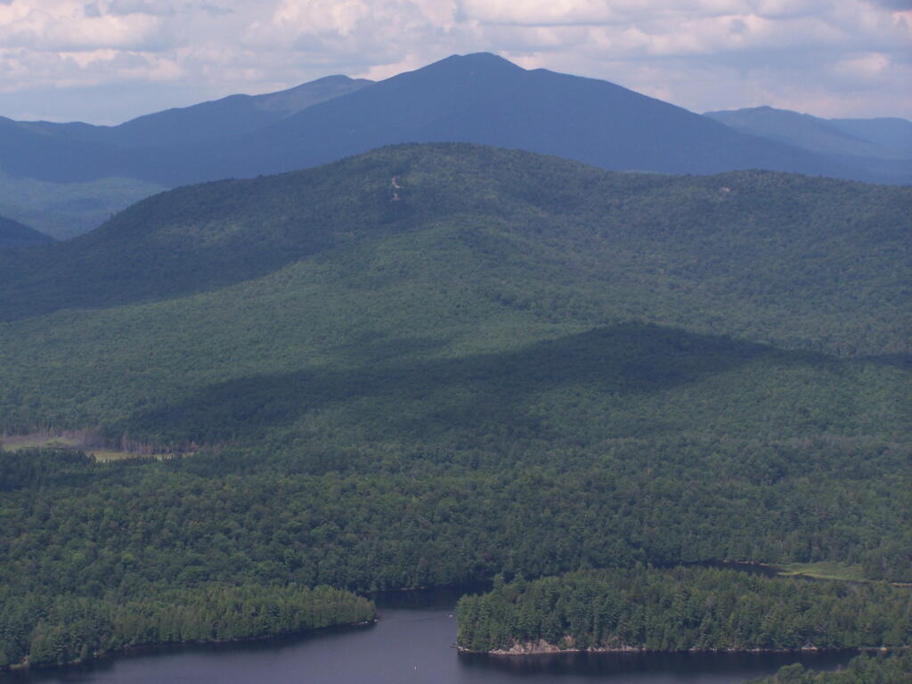
While certainly not a surprise to most observers, the Catskill Mountains are largely wild, without much housing development or agriculture. Tree covered areas are a deeper green, while cleared areas are white or clear.
After studying the methods quite a bit, I’ve determined there is no real easy way to find peaks on mountains and report their exact elevation in QGIS. The best method I could come up with was to figure out the median point in the elevation for the map, then use that to isolate “mountains” and from there polygonize, create zonal statistics for each polygon, crop the DEM layer to each polygon then select the pixel that matched the peak. This can be done, but I couldn’t figure out how to automate it easily using the Graphical Modeler, so I would have to write a full plugin to do it. I decided it wasn’t worth the effort. In most cases, I didn’t care about the exact peak, and it would just be easier to add peaks to my maps on a case-by-case basis using a point layer with labels queried against the DEM layer.
Make Your Maps in QGIS but use R and Tidycensus to Generate Census Shapefiles 🗺
Why choose when you can have it all? Seriously, QGIS makes it easy to move labels as you like and do the styling of the Shapefile or GeoPackage you generate in R with tidycensus and sf.
With the above R code, it will generate a GeoPackage (use extension .gpkg) or Shapefile (use extension .shp) you can use to make your map in QGIS. Then in QGIS if you want to simplify the output, you can use a geometry generator in the styles:
simplify($geometry,0.003)
Or you can specify the simplification in the R script when you run get_acs(), as it is a wrapper around the tigris package:
I like this PHP geocoding script I wrote to use with SAM, as it’s so simple, just six lines. Should I have used Python or Perl? Probably and it would have probably been 3 lines in Python or in case of Pathologically Eclectic Rubbish Lister probably one line. Basically you call this on command line with a text file list of addresses, and spits out a CSV file with the addresses followed by the coordinates from the NY State Address Management system. Most other states have something similar, as it’s kind of important that the fire truck and your Uber show up at the right house.
Louise E. Keir WMA – Albany
Gas Springs State Forest – Allegany
Hanging Bog WMA – Allegany
Karr Valley Creek State Forest – Allegany
Phillips Creek State Forest – Allegany
Mccarthy Hill State Forest – Cattaraugus
Rock City State Forest – Cattaraugus
Frozen Ocean State Forest – Cayuga
Whalen Memorial State Forest – Chautauqua
New Michigan State Forest – Chenango
Perkins Pond State Forest – Chenango
Mariposa State Forest – Chenango-Madison
Macomb Reservation State Forest – Clinton
Livingston State Forest – Columbia
Taylor Valley State Forest – Cortland
Trout River State Forest – Franklin
Beartown State Forest – Lewis
Frank E. Jadwin State Forest – Lewis
Grant Powell Memorial State Forest – Lewis
Indian Pipe State Forest – Lewis
Sand Flats State Forest – Lewis
Charles E. Baker State Forest – Madison
Popple Pond State Forest – Oneida
Rome Sand Plains Unique Area – Oneida 1
Huckleberry Ridge State Forest – Orange
Roseboom State Forest – Otsego
Gates Hill State Forest – Schoharie
Petersburg State Forest – Schoharie
Sugar Hill State Forest – Schuyler
Brasher State Forest – St. Lawrence
Helmer Creek WMA – Steuben
Calverton Pine Barrens State Forest – Suffolk
David A. Sarnoff Preserve – Suffolk
Otis Pike Preserve – West – Suffolk
Rocky Point Pine Barrens State Forest – Suffolk
Bashakill WMA – Sullivan
Hickok Brook State Forest – Sullivan
Mongaup Valley WMA – Sullivan
Roosa Gap State Forest – Sullivan
Wolf Brook Multiple Use Area – Sullivan
Wurtsboro Ridge State Forest – Sullivan
Hammond Hill State Forest – Tompkins
Potato Hill State Forest – Tompkins
Witch’s Hole State Forest – Ulster
I bet a lot of people who incorrectly cast coordinates in Eastern NY as a integer rather then a floating point number will end up in a field north of Leggs Mills Road in Saugerties.