“I could come up with an interesting idea for a blog post, or a could just write a line or two to connect to a government GIS server, and call that a blog post.”
Earlier today I posted a Leaflet Map showing the current Satellite Image from NOAA’s GEOS-East derived product, the GeoColor. It’s nice but to look really attractive you need to increase the brightness and saturation. If you want a 1920×1080 image that looks nice that you can download, you can use this python code. This ARC GIS Image Server is relatively straightforward to work with — supply a bounding box in Web Mercator, size and a few other parameters and it will spit back the image you want.
import requests, io
from PIL import Image, ImageEnhance, ImageDraw, ImageFont
from datetime import datetime

# new york - new england
url = "https://satellitemaps.nesdis.noaa.gov/arcgis/rest/services/MERGED_GeoColor/ImageServer/exportImage/exportImage?bbox=-9011008.3905,4747656.7008,-7345292.6701,6195679.7647&size=1920%2C1080&format=jpgpng&transparent=false&bboxSR=3857&imageSR=3857&f=image"

# full usa
#url = "https://satellitemaps.nesdis.noaa.gov/arcgis/rest/services/MERGED_GeoColor/ImageServer/exportImage/exportImage?bbox=-14401959.1214%2C2974317.6446%2C-7367306.5342%2C6447616.2099&size=1920%2C1080&format=jpgpng&transparent=false&bboxSR=3857&imageSR=3857&f=image&fbclid=IwAR1HvlVi55Bd933eOhM-Cvou2JgPdKAlcp2go4f8B5pqcioAPvcJyfYT0BA"

response = requests.get(url)
image_bytes = io.BytesIO(response.content)
img = PIL.Image.open(image_bytes)

enhancer = ImageEnhance.Color(img)
img = enhancer.enhance(2.5)

enhancer = ImageEnhance.Brightness(img)
img = enhancer.enhance(1.2)


img.save('/tmp/latest_image.jpg')
When using a projected coordinate system, it turns out you can calculate distance with a very simple lambda function. Beats that ugly haversine formula you have to use with World Geodetic System 1984.
lambda xa, ya, xb, yb : math.sqrt((xb-xa)**2 + (yb-ya)**2)
Here is the equalivent with WGS 84 (written as a Lambda):
Maybe I’m a bad person for saying this, but I generally just accept that there is 1610 meters in a mile and 2.6 million square meters in a square mile. #roundingworks #gosueme
Math like this will probably be a bad thing if you are aiming a missile to hit a target thousands of miles away but for ordinary life, i think it’s quite fine. I use 1610 meters a mile, because it’s easier to round up — a half mile then becomes 805 meters, a quarter mile 402.5 miles, a tenth of a mile is 161 meters. If you rounded down to 1609 meters, that math becomes a lot harder to do in your head.
How did I not know that QGIS can natively open Shapefiles in ZIP files?
OpenTopography provides community access to high-resolution, topography data, related tools, and resources … FOR FREE! OpenTopograhy.org Sponsored by Regrid.com Leading provider of land parcels and location context data for your maps, apps, and spatial analysis.
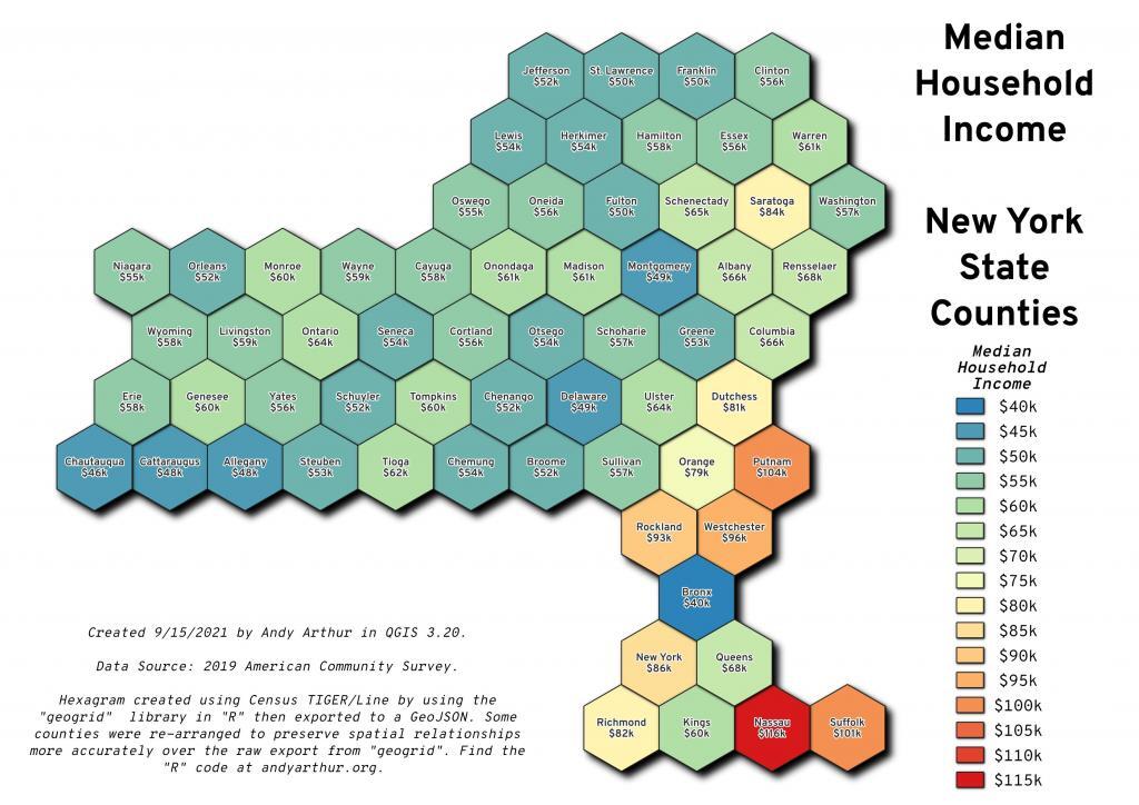
Mr. Bailey’s geogrid R-library is pretty neat. You will need to install the “R” language along with geogrid and sf libraries, which you can do with install.packages(‘geogrid’). After installing R and the library, the code to create a hexagram is pretty simple, although you will want to tweak the output a bit in QGIS after creating the computer-generated hexagram.
# required libraries
library(sf)
library(geogrid)

# load geojson shapefile
df <- st_read( "/tmp/nyco.geojson")

# iterate through seed values 1 to 10 to compare which
# is the best output of hex file (optional, but various seeds
# can improve the output)

for (i in seq(1,10)) {
# calculates hexgrid as a foreign object
  tmp <- calculate_grid(shape = df, grid_type = "hexagonal", seed = i)

# Convert foreign object to an spatial dataframe
  df_hex <- assign_polygons(df, tmp)
  df_hex = st_as_sf(df_hex)

# save spatial dataframe as geojson
  st_write(df_hex, paste("/tmp/nyco_hex_",i,".geojson", sep = "") )
}