R is a programming language and free software environment for statistical computing and graphics supported by the R Core Team and the R Foundation for Statistical Computing. It is widely used among statisticians and data miners for developing statistical software and data analysis.
Here is an R function that takes a LINESTRING or touching MULTILINESTRING and returns a series of points along the line string at each mile, much like the “tombstone” mile markers along an expressway. This is helpful for making maps when you want to plot distance for hikers or drivers looking at their odometer of their car. It has the option to “reverse” the linestring so you can have the points going the opposite direction of the linestring, such as south to north. The code can be modified for quarter mile points or however you find useful.
library(tidyverse)
library(sf)
library(units)

make_milepoint <- \(linestring, reverse = FALSE) {
  # make sure were using a projected coordinate systm
  linestring <- st_transform(linestring, 5070)

  # merge parts together into a multilinestring
  linestring <- linestring %>% group_by() %>% summarise()

  # if multiline string, then attempt to join together
  # this will raise an exception if the linestring is not contiguous
  if (st_geometry_type(linestring) == 'MULTILINESTRING')
    linestring <- st_line_merge(linestring )

  # reverse the string if we want to
  # go from the other end
  if (reverse)
    linestring <- st_reverse(linestring)

  # length of string in miles
  linestring.distance = st_length(linestring) %>% set_units('mi') %>%
    drop_units()

  # percent of string equals each mile including start and end
  linestring.sample.percent <- seq(0, 1, 1/linestring.distance) %>% c(1)

  # sample line string, convert multi-points to points, convert to sf
  # add a column listing the mile-points, round to two digits
  st_line_sample(linestring, sample = linestring.sample.percent) %>%
    st_cast('POINT') %>%
    st_as_sf() %>%
    mutate(
      mile = round(linestring.sample.percent * linestring.distance, digits = 2))
}
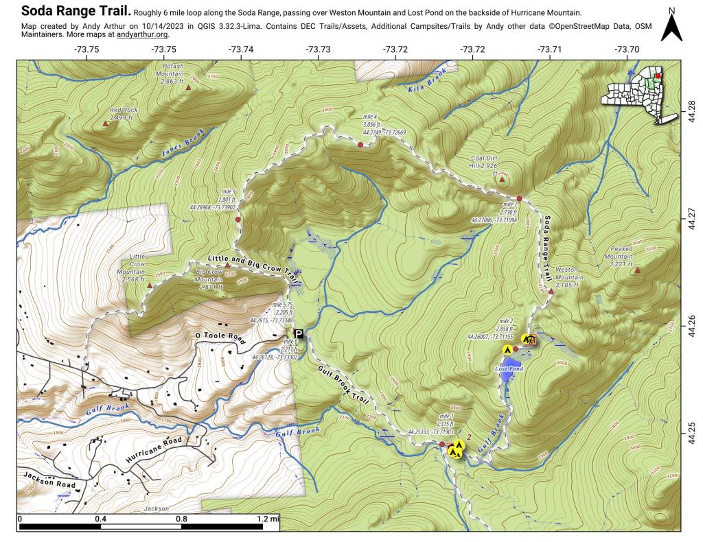
Here is an example of the 1 mile points it outputs along Piseco-Powley Road.
And here is a static (paper) map I created using this code plus adding coordinates and elevation for this hiking map.
Been learning about Apache Arrow for loading and processing extremely large datasets in R quickly without having to set up and use something like a PostgresSQL database. DMV vehicle file, you know what I'm thinking.
The R code is fairly simple — just grab the JSON from the server and use purrr to map over the various styles. The returned tibble contains the value returned from the server, along with the label and fill color.
# this builds a dataframe of styles/colors from feature server
feature.info <- jsonlite::read_json('https://services.arcgis.com/cJ9YHowT8TU7DUyn/arcgis/rest/services/AirNowLatestContoursCombined/FeatureServer/0/?f=pjson')
style <- map(feature.info$drawingInfo$renderer$uniqueValueInfos,
    \(x) {
      tibble(value = x$value %>% as.numeric,
             label = x$label,
             color = rgb(x$symbol$color[[1]], x$symbol$color[[2]], x$symbol$color[[3]], x$symbol$color[[4]], maxColorValue = 255))
    }
  ) %>% list_rbind()
I keep telling myself that I should do more Python programming as it’s the future and R is a dying language. R isn’t the most popular language compared to Python.
But the thing is Python remains far behind R when it comes to map making and graphics. And there is a ton of useful packages out there for R, sometimes much better packages for R then Python especially when it comes to graphics and light manipulation of data, especially Census data. PANDAS might be better for heavy lifting then tidyverse but for many things the tidyverse is simpler.
Yet I concede R is a like adopting the Macintosh System 7 platform decades ago in the era of Windows 95. Your simply not using what the masses are using and you are somewhat locked out of benefits of a popular platform. Moreover, the underlying code in R is often slow and inefficient, with a legacy of 50 year old designs unlike the relatively modern clean and elegant of Python. Much like Macintosh System 7 compared to Windows 95. Macintosh System 7 did a lot of things good in graphics and user interface but the underpinning were a hot mess of hacks built on code from the early 1980s. Windows 95 had protected memory and preemptive multitasking while System 7 was stuck in the era of shared memory and cooperative multitasking.
But R is different than Macintosh System 7. R might be creaky and old but it’s actively maintained and unlikely to be killed off with a single shot by a corporation like Apple did with Macintosh System 7 with the release of Mac OS X. R programming will last forever even if it eventually dies out to Python as it’s open source and not controlled by a profit seeking corporation. Old R code is unlikely to stop working, as there is enough existing code base that interpretive environments are likely to be maintained just like how GNU FORTRAN still is a thing despite little new FORTRAN code written anymore.
Yet my bigger fear is that every time I use R programming language not only am I not writing truly future compatible code, I’m not practicing a skill that is beneficial for my future. I’ve read a lot of books on Python code and I’ve written a lot of Python but the way to be truly good at something is to use it a lot and practice. It’s great to be a skilled R programmer but if Python is the future it’s what for naught. Yet, I constantly find when I write code in Python the weakness of the graphics, geospatial and even data wrangling capacities come back to bite my compared to what I can easily do in R no matter how much research I do into libraries and best practices. And that troubles me to keep going back to the second fiddle known as R programming.